
by Noémie Globus
A century after the discovery of cosmic rays, delving into their mysteries remains a primary focus of high-energy astrophysics. Cosmic rays consist of energetic particles propagating through interstellar and even intergalactic space, and are characterized by an energy spectrum extending over at least eleven orders of magnitude, from ~1 GeV (giga-electronvolt, a commonly used unit of energy in astrophysics) to extreme energies of about 1011 GeV (for comparison, the mass of a proton when converted to an equivalent energy via E=mc2 is just under 1 GeV—so those highest-energy cosmic rays have about the energy of a fastball packed sometimes into one elementary particle!).
The particles at the more extreme end of the cosmic-ray spectrum are called Ultrahigh Energy Cosmic Rays (UHECRs), and are the cosmic rays with energies greater than 1 exa-electronvolt (EeV), which is 109 GeV (cosmic rays composed of very high energy photons were previously covered in a post from Apr 2015 discussing the future Cherenkov Telescope Array, and with regard to their sources in galaxies in a post from Nov 2015).
When a cosmic-ray interacts in the atmosphere, it produces what's called an air shower (see Figure 1), which is a cascade of ionized particles and electromagnetic radiation. A 1011 GeV cosmic ray produces over 100 billion particles in the atmosphere! The lower-energy secondary particles, as well as the UV light emitted by the interaction of these particles with air molecules, are detected from the ground by giant air shower arrays and their fluorescence telescopes. The flux of the original incident UHECR particles is very low (around one particle per square kilometer per year at 1 EeV, to one particle per square kilometer per century at 100 EeV).

Two giant air-shower observatories are currently detecting UHECRs: the Pierre Auger Observatory (hereafter “Auger”) in Argentina in the Southern hemisphere and Telescope Array in Utah in the Northern hemisphere. UHECRs have been extensively observed over the last decade and tens of thousands of cosmic rays have already been detected.
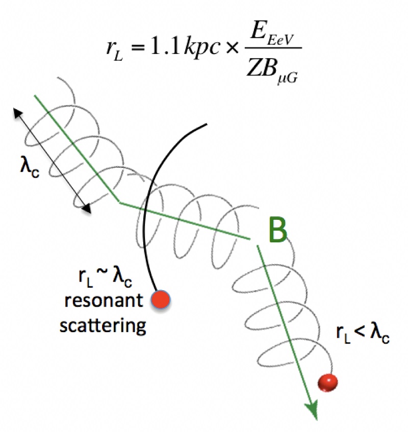
However, the sources of the UHECRs have yet to be pinned down. As cosmic rays are charged particles, their paths curve as they propagate through a magnetized Universe (as do all charged particles in motion under the influence of magnetic fields) and therefore, the direction from which they arrive here does not point straight back to their source. They are deflected on their way to the Earth by the intervening galactic and intergalactic magnetic fields (GMFs and IGMFs, respectively). Moreover, the cosmic rays are scattered by magnetic field irregularities, and most efficiently when these irregularities are of the size of their gyroradius which is the radius of the circle they would make in a constant magnetic field, given the particle’s velocity, as illustrated in Figure 2 below. After many scatterings, the memory of the initial direction is lost and the cosmic rays enter the diffusive regime.
The Auger dipole anisotropy
The global analysis of UHECR arrival directions yields a clear signature of a large-scale angular anisotropy, or unevenness, in the source direction of particles above 8 EeV with an amplitude that was larger than previous observations of cosmic rays had led astronomers to expect (on the order of ~7%), with the amplitude increasing with energy (Auger Collaboration, Science, 2017, and ApJ, 2018). What's more, the anisotropy resembles a dipole, with more particles arriving from one hemisphere and fewer from the other.

At energies of 8 EeV and above, cosmic rays are almost certainly extragalactic in origin. As a comparison, the gyroradius of a 1 EeV proton in a magnetic field with a strength of about a microgauss (typical for the Milky Way—for comparison, the Earth’s magnetic field has a strength of about half a Gauss) is of the order of a kiloparsec (about 3300 light years).
The GMF has a lensing effect and some directions would be better connected to Earth than others. To probe this further, we introduce a new term called "rigidity": the deflection of a cosmic ray in a magnetic field depends on the ratio of the particle's energy, E, to the particle's charge, Z. For illustration, Figure 4 shows cosmic ray trajectories for a rigidity value (E/Z) of about 3 EV, coming from the Galactic center direction and from the anticenter direction (i.e., opposite the center towards the edge of the Galaxy), respectively.

The dipole anisotropy: a signature of the local large scale structure?
Now we must probe how the observed UHECR dipole anisotropy is set by the size of the UHECR-observable Universe. The cosmic ray horizon, which is the largest distance that the UHECRs can propagate at a given energy, depends on their diffusion coefficient in the IGMF and on their mean free path in the photon backgrounds. The more intense the magnetic field, the less cosmic rays can diffuse out to far distances. We calculate the UHECR horizon assuming a purely turbulent IGMF, with a root mean square value (intensity) between 0.01 and 10 nanoGauss (nG, or 10^-9 G). Different magnetic field strengths probe different cosmic-ray magnetic horizons, as seen in the left panel of Figure 5.
Then, for different values of the IGMF (which give different values of the UHECR horizon), we calculated the UHECR anisotropy expected from the Universe's large-scale structure (LSS), first using the power spectrum of density fluctuations (Globus & Piran, 2017), and then using the density field predicted by cosmological constrained simulations (Globus et al. MNRAS, 2019) and showed how the amplitude and direction of the dipole depends on the strength of the IGMF.
A 3D view of the density field of the local universe we used in our calculations is shown by the right panel of Figure 5.

The animated Figure 6 show the sky maps obtained for different values of the IGMF (and hence different horizons). This is what an observer sitting outside the Galaxy would see. The dipole component of each sky map is figured by the black dot. The amplitude of the dipole component is indicated next to the black dot. One can see that for large horizons (small IGMF) the direction of the dipole coincides with the CMB dipole, whereas for small horizons (large IGMF) it coincides with Local Structures (the closest significant over-density being the Virgo cluster, close to the North Galactic pole on the sky map). The amplitude of the dipole increases as the horizon shrinks, which is natural since a smaller horizon means an enhancement of the signatures of local structures.
However, to compare with the actual observations (Figure 3) one has to consider the effect of the GMF. The right panel of animated Figure 6 show the anisotropy after lensing by the GMF, using the most advanced magnetic field model currently available (Jansson and Farrar 2012). This is what an observer sitting inside the Galaxy would see. Compare now the dipole direction observed by Auger, indicated by the red circle, with the black dot belonging to the dipole we calculated. One can see that as the horizon shrinks the dipole component of the sky map become more and more compatible with the observations. As Auger composition analyses suggest a composition becoming gradually heavier above a few EeV, we performed the calculations for nitrogen, since intermediate mass nuclei seems to dominate at this energy.
For these calculations, we vary the rms intensity of the IGMF, as indicated on the left top corner. The direction and amplitude of the dipole component is shown by a black dot.

In conclusion, we find a dipole amplitude and direction expected from the LSS consistent with observations when the IGMF is quite large, a few nG. These are preliminary results and further studies that will take into account the uncertainties on the GMF parameters are planned.
This is highly suggestive—and indicates that for the first time in over a century, scientists are now finally getting some insight into the mysteries surrounding the origin of these cosmic messengers from afar.
Further reading (arXiv links where available):
Cosmic-Ray Anisotropy from Large Scale Structure and the effect of magnetic horizons (Globus et al. 2018)
Observation of a large-scale anisotropy in the arrival directions of cosmic rays above 8 × 10¹⁸ eV (Auger Collaboration, 2017)
Large-scale cosmic-ray anisotropies above 4 EeV measured by the Pierre Auger Observatory (Auger Collaboration, 2018)
")